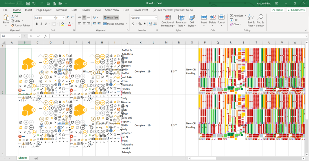
You’ve carefully selected the data you need from a website and pasted it to Excel. Far too often, the result looks messy, various objects are included (hyperlinks, icons/images, etc.), wrap text explodes the row height, the text’s font and size rarely matches what you are looking for. You all know this looks ugly. For those who don’t know, please see the image below.

There are many ways to address this. In this article (part 1 and part 2) I will share with you methods I know.
Option 1: Clean-up
Step 1: Remove the objects
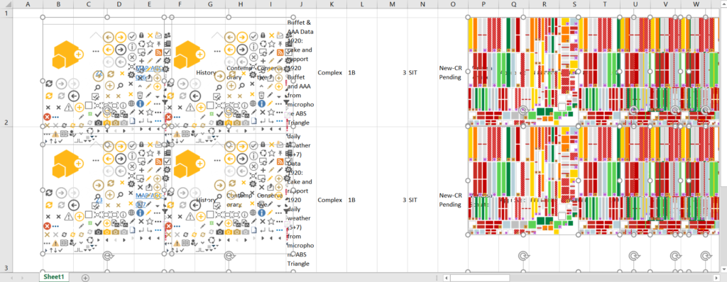
On the ‘Home’ tab click on ‘Find & Select’ then ‘Go To Special…’. In the pop-up window select ‘Objects’, then click OK. Text was pasted into the cells and cells are part of the grid. All the objects that are not part of the grid will be selected. This is how it looks.

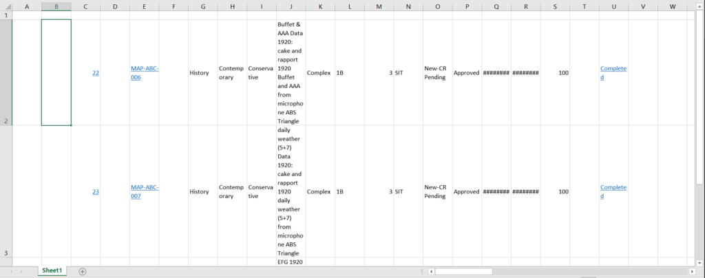
Verify all unwanted objects are highlighted. Press ‘Delete’ button on your keyboard to remove all the objects. Now you can see the data you need, but it still looks ugly.

Step 2: Remove the formatting
To be able to work with all cells at once, select them all by clicking on the ‘Select All’ button – a grey area above ‘1’ (row button 1) and to the left of ‘A’ (column button A) – or using a keyboard shortcut Ctrl+A. Now that you have all the cells selected, on the ‘Home’ tab pick a font and font size you like. Also on the ‘Home’ tab click on ‘Wrap Text’ button once or twice until all rows go back to their initial height. If necessary, you can also remove the borders (‘Home’ tab -> Borders -> No Border) and cells’ background colour (‘Home’ tab -> Fill Color -> No Fill). Now your data looks much better, but you are not done yet.

Step 3: Remove the hyperlinks
Unless you need to keep the hyperlinks for whatever reason, I suggest removing them to have the source data clean and ready for use. While all cells are still selected, right-click with your mouse anywhere on the grid to open the context menu. Choose ‘Remove Hyperlinks’ to finish cleansing the data you need.

Optional: You can choose to resize the columns to be able to see the contents. Also, columns with no data can be deleted and column names added. When your data is ready, you can start working with it.
Option 2: Paste Special
Before pasting anything to Excel (if you pasted already click ‘Undo’ or Ctrl+Z on the keyboard to return to empty grid), choose to paste only text from everything you copied. On the ‘Home’ tab click on the ‘Paste’ dropdown arrow. From ‘Paste Options’ click on the button ‘Match Destination Formatting’.

I know! Sorry, I made you read through all the steps of Option 1. Of course, being neat is easier and faster than appear fast at first and then cleaning the mess.
In part 2 I will talk about linking to the web to get updated info at any time without needlessly copying and pasting.


