Who doesn’t want to build Excel Pivot Tables fast and easy, and without rework? If you encounter difficulties, error messages and warnings, this article is for you.
In the article “What is a Pivot Table?” I discussed the importance of having a quality data source. Any journalist, police officer or data scientist should trust their sources. The source is essential to anything you do. Think of the best restaurant you know. Do they take seriously where they source their products? This is the classic garbage in – garbage out.
If you follow the 5 rules below, you will build Pivot Tables faster and therefore save valuable time for analysis of the data:
.
1. Ensure all columns have headers
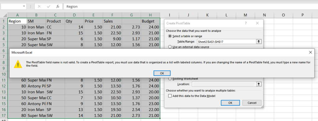
That is essentially the name of your field/column. When working with Pivot Tables you work with those names. Having an empty column header will result in an error message that will prevent creating your Pivot Table.
There are cases when you insert a column say, to help with a calculation step, or for a multitude of other reasons. Every time you do that, always name your new column to avoid an error message.
2. Avoid duplicate column headers
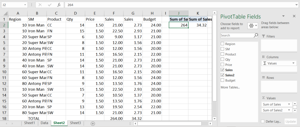
Say, you added the calculation column, didn’t put too much thought to it and copied the column name from the left. If you have a duplicate column name, Pivot Table will be built with no errors, but subsequent duplicate names will be assigned a sequence number in addition to the original name. For example, if you have 2 columns named Date, Excel will assign “Date” to the first Date, “Date2” to the second occurrence and so on. Make sure you give a meaningful and unique name to each column to easily identify them when designing your Pivot Table.
3. Avoid empty columns and/or rows
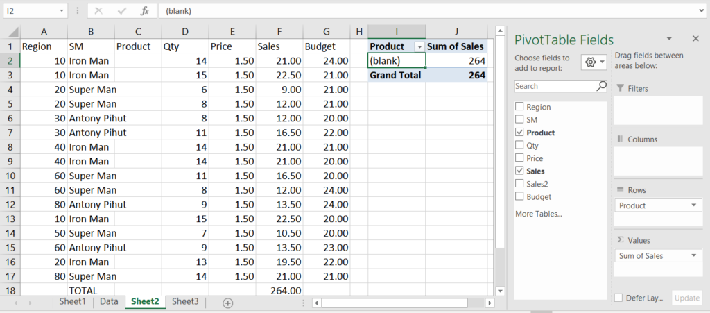
This is has similarities with the point above, as the break will not have header for sure. But even if you added a name as suggested above, your Pivot Table will show an ugly (blank) if the field is used in one way or another.
There can be a variety of reasons why data might have breaks. One that comes to mind is for readability purposes someone might decide to add a break. Either an inserted empty column to visually separate, for example Actual from Budget, or an empty row to have breaks between months. Another reason might be pre-formatting of systems data extracts with page breaks. Empty columns with headers will not prevent you from creating a Pivot Table. Though I advise using continuous uninterrupted data sets in Excel.
4. Ensure consistent data in columns
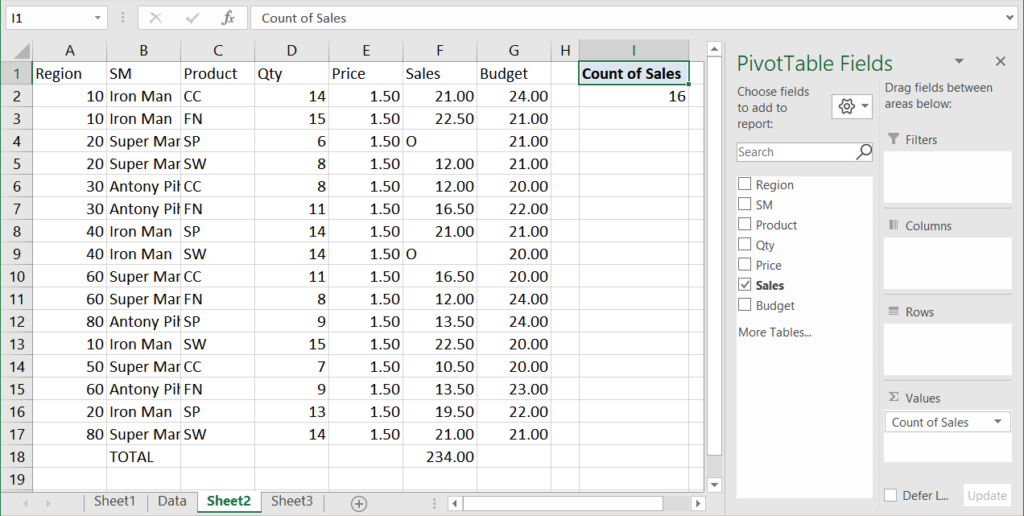
Being consistent, pays off! Your column header describes or implies the data type in that column. A column with numbers must contain numbers. Pivot Tables are a very powerful tool with fast aggregations among other features. Those aggregations will not work as intended if a number column added to Values contains empty cells or cells with text. As you drag a column with numbers into the Values area of a pivot table, it will auto detect COUNT operation instead of SUM.
Same applies to dates. A column with dates must contain dates. Otherwise Pivot Table will not be able to group data by months and years, etc.
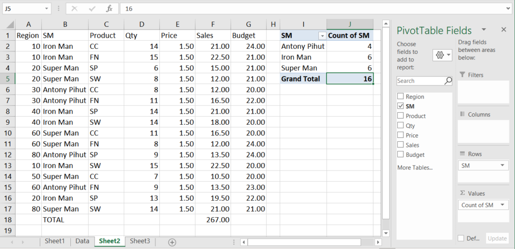
A column with text may contain any sort of data including numbers and dates, but don’t expect to be able to do any math operations with those values. The entire column will be treated as text and no aggregations will be applied. Text data is good for Rows, Columns and page/report Filters in Pivot Tables. If used in Values, it will only count the occurrences of the records in that column, which can also be useful if this is what you a trying to analyze.
5. Use Tables to help with all of the above
In the above screenshots the source of the Pivot Table is just a range of cells A1:G17. I say ‘just a range’ because there is another way of organizing your data source. Using Tables in Excel will not only help you with the pitfalls described above, but it will also bring you many other benefits. If interested please follow this link to learn about benefits of using Tables in Excel.


